Parabolic Reflectors
A configuration often used for very short wavelengths is the
Cassegrain antenna, (called a "telescope" at optical
frequencies). It utilizes a hyperbolic subreflector to
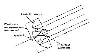
intercept
reflected waves before their normal focal point
and re-reflect them back to a rear
mounted head unit. The main
advantages are that it has a slimmer
profile than the traditional front
fed designs, the feed head is better
shielded from noise. The
main disadvantage are the added expense of the hyperbolic subreflector,
and signal blocking that it causes. As a general rule, if the
diameter of the main reflector is greater than 100 wavelengths,
(and if there exist sufficient finances) the Cassegrain system
is a contending option.
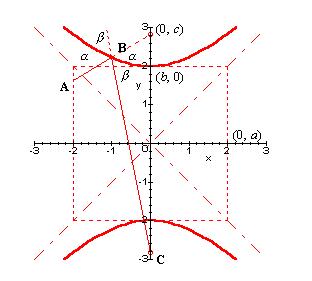
A hyperbola is defined by
the equation:y^2/a^2 +x^2/b^2=1, where a^2 + b^2 =
c^2
and 2c is the distance between the
two foci. Above, we have a
plot of the hyperbola, y = sqrt(4+x^2) . In our
antenna system it is required that
we position one hyperbolic focus so
that it coincides with the
parabola's focus.
A typical ray will approach the hyperbolic focus on a path as
represented by AB. Encountering the hyperbolic surface at angle
alpha, it is reflected at an equal angle and it's new path, as
represented
by BC, takes it to the other hyperbolic focus. The proof that this
system works is similar to our earlier one concerning parabolas. Here,
however, we will work with an equation like:
arctan((a+c-x)/x)-arctan((c-y)/x)=2arctan((a^2/b^2)(1/sqrt(a^4x^2/b^2))),
which will take time to crack. I'll get around to it some day.
Although this proof may
be considered crucial to the success of this paper, I will settle
for less. I have written a Maple routine which will show
that the Casegrain system works for any particular angle the user selects.
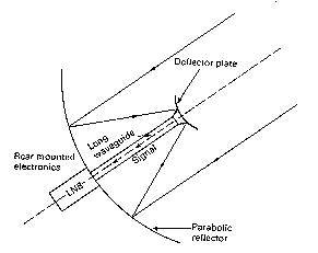
The configuration above uses a
wave guide to transport signals
to/from the feed head. This design is
often called a "backfire" type
antenna. The main reason for placing
the feed head near the subreflector
is that a shorter focal distance
gives the system a greater field
of view. It is easy to visualize small deviations in the incoming
parallel rays still successfully reaching the feed horn with this
design. With the focal distance extended to or beyond the dish,
the restriction on the incident angle is greater and so the field
of view is reduced. It should be noted that a reduced field of
view corresponds with an increased magnifying power of the system.
High power telescopes have large aperture sizes and large focal
distances.

Here is a real-life
example of a Cassegrain
system. The focal point of
the paraboloid is slightly
behind the secondary
reflector. After reflection
from the hyperbolic surface,
the rays converge on the feed
horn, which
extends slightly past the plane formed by the rim of the dish,
as is barely visible in this photo. Below we have another picture
of this antenna. Radiation gathered by the 12 foot
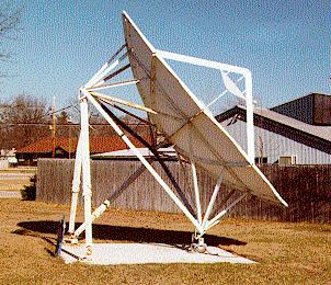
dish is focused
to within a couple inches,
where it is collected by the
feed horn. The focal length
is about 8 feet. We note that
the obstruction presented by
the secondary reflector is
not
significantly greater than that from a conventionally placed feed
head.
It is interesting to note that one of the highest gain antennas
in the world (148 dB) is a paraboloid. This is the 200 inch Mt.
Palomar telescope in California. The very short wavelength of
light rays causes such a high gain to be realizable. (The 300 meter reflecting antenna at Arecibo is not parabolic,
but shperical in shape.)
The Gregorian antenna differs from the Cassegrain in that the
hyperbolic sub-reflector is replaced by one with an elliptical
surface. Invented by the Scotsman James Gregory in 1661, the
reflecting telescope was first successfully constructed by Newton
in 1668 and only became an important research tool in the hands
of William Herschel a century later. This geometry allows for
a proportionately smaller secondary reflector, making the configuration
efficient at longer wavelengths. However, the advantage of small
profile is somewhat diminished form the Cassegrain design.

An ellipse is defined by the
equation y^2/a^2+x^2/b^2 = 1, where the foci are
located at y = +-sqrt(a^2-b^2). Above we have
a sketch of the ellipse . The foci
are located at (0, +-sqrt(7)). For the
Gregorian system to
work, it is necessary that one of the foci be coincident with
the parabola's focus. Then a typical ray entering as AB encounters
the ellipse surface at angle alpha and is reflected at an equal
angle.
It's new path is represented by BC , and takes it to the other
elliptic
focus. I have not yet been able to prove that alpha = beta. The
proof requires
that I solve an equation similar to:
(y-c)/x = 90-(90-arctan(x/2c)),
which I will someday find time for. We have another Maple program for the
Gregorian system - and this will have to suffice for now.
You can view or download the Maple programs by clicking on the
appropriate link below. They are pretty cool. Or you can bypass the
programs (if you've already seen them or if programing scares you).
Cool Maple Programs.
Program bypass