A modern textbook problem goes like this: students are provided
a real world manifestation of a functional relationship, complete with a
collection of data. A graphing calculator is used to plot data and to impose a
curve through the points. The "regression" technique is generally seen by the
student to be a sort of proof that the particular relationship exists between
the variables.
Having arrived at the desired and presumably concluding step,
students are satisfied with their accomplishment (or at least relieved) and
resist further inspection. They avoid the paradox that other students have
obtained equally professional looking displays while using the ‘wrong’
functional choice; a cubic rather than a quadratic regression for example. The
teacher or the text is expected to provide a judgment. An explanation is
actually required.
| I use an example of my own. I
tell the class that I had stuck my head into the sink at home to get a
drink and noticed an interesting curve. (This line guarantees a chuckle,
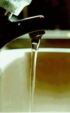
but I want to apply math to ordinary situations). I show this picture on
the overhead and point out that water falls in a laminar column of
decreasing radius. I suggest that the vertical edge looks somewhat like a
parabola, and that we might use quadratic regression to chart it on a
calculator. The idea is acceptable. The curve is certainly not linear, and
students are familiar with parabolas. |
|
The varying radius of tap water would be difficult to
measure directly. I recommend that we use a photograph. I also advise us
to use syrup rather than water. I ask them to speculate during the
experiment as to why syrup might be better.
As a chosen student empties syrup into a bowl, I snap a half
dozen pictures with a digital camera and distribute printouts to small groups.
Each student fills in a table relating distance fallen to radius.
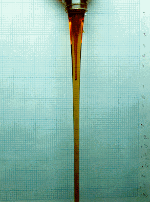 |
I use graph paper as a backdrop
to eliminate some of the measurement problems. As you can see, the boxes
seem to get smaller near the bottom, where they are farther from the
camera. I keep the bottle close to the backdrop to reduce other errors
resulting from the angle of vision. After tabling data, students chart the
points on a graphing calculator and impose a second order polynomial curve
through them. They are then sufficiently pleased/relieved. I continue by
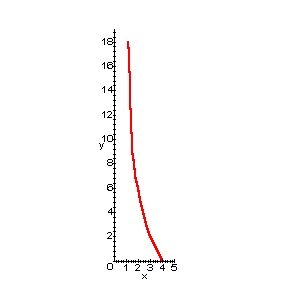
presenting tabled measurements and a computer graph of my own
results. |
| Via inquiry, we decide that our
plots are inverted representations because our conventional machines place
positive numbers in the first quadrant. Our curves are also bumpy,
illuminating the difficulty of measuring this way. |
 |
I show my tabulated data on the overhead:
|
Distance
|
Diameter
|
Radius
|
|
0
|
8.1
|
4.05
|
|
1
|
7.0
|
3.50
|
|
2
|
6.0
|
3.00
|
|
3
|
5.3
|
2.65
|
|
4
|
4.8
|
2.40
|
|
5
|
4.4
|
2.20
|
|
6
|
4.0
|
2.00
|
|
7
|
3.6
|
1.80
|
|
8
|
3.3
|
1.65
|
|
9
|
3.1
|
1.55
|
|
10
|
3.1
|
1.55
|
|
11
|
2.9
|
1.45
|
|
12
|
2.9
|
1.45
|
|
13
|
2.7
|
1.35
|
|
14
|
2.7
|
1.35
|
|
15
|
2.7
|
1.35
|
|
16
|
2.6
|
1.30
|
|
17
|
2.5
|
1.25
|
|
18
|
2.4
|
1.20
|
Selecting three representative points from the list above, I
invoke Lagrange's formula for interpolation, producing a quadratic function,
which includes the points*.
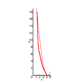 |
I used Maple to produce the plot
shown here, with the curve passing through the selected points. We have a
pretty good fit. Selecting other points for the interpolation may have
resulted in a more accurate representation.
*I don't expect them to know how to do this yet, but they can see it
without threat. This is a radical break from routine, (packaged within the
firmware).
|
I used the same method to look for a polynomial of degree four.
I selected points (1.2, 18), (2.4, 4.0), (2.65, 3.0), (3.0, 2.0), (3.5, 1.0).
Part of the Maple code is shown below.
|
>
Lmo:=(x->((x-2.4)*(x-3)*(x-3.5)*(x-4.05))/((1.2-2.4)*(1.2-3)*(1.2-3.5)*(1.2-4.05)));
>
Lm1:=(x->((x-1.2)*(x-3)*(x-3.5)*(x-4.05))/((2.4-1.2)*(2.4-3)*(2.4-3.5)*(2.4-4.05)));
>
Lm2:=(x->((x-1.2)*(x-2.4)*(x-3.5)*(x-4.05))/((3-1.2)*(3-2.4)*(3-3.5)*(3-4.05)));
>
Lm3:=(x->((x-1.2)*(x-2.4)*(x-3)*(x-4.05))/((3.5-1.2)*(3.5-2.4)*(3.5-3)*(3.5-4.05)));
>
Lm4:=(x->((x-1.2)*(x-2.4)*(x-3)*(x-3.5))/((4.05-1.2)*(4.05-2.4)*(4.05-3)*(4.05-3.5)));
>
Pm4:=(x->18*Lmo(x)+4*Lm1(x)+2*Lm2(x)+1*L3(x)+.00001*Lm4(x));
> ch1:=plot (Pm4(x), x=0..5):
> display ([ch1, ch3]);
|
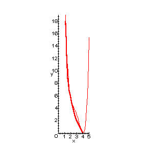 |
Now this curve fits much better. It's not perfect, but there is
nothing in the graph to contradict the notion that distance fallen is
proportional to the fourth power of the radius, (that is if we admit that all
radii greater than the initial one are meaningless). We might claim that
evidence shows the direct relationship and point to this display as our proof.
But of course that's not right.
So why are we doing it? That is the important
question and the essence of these kinds of exercises. It is also the most easily
neglected issue - but what should we assess if this point is missed?
I submit to the students that if we need a mathematical model
of this particular column of syrup, we have one. We could use a linear
model for small sections, but the quadratic fits the whole column better. The
fourth degree fits better still, but parabolas are familiar and (hopefully)
friendly curves. We could maybe use one for whatever calculations we might need
to do with this example.
But we might be able to derive a model for all similar
effusions. If we could link radius to distance from the spout in some general
way, we may have a better handle on all sorts of situations. I present the
following in front of the whole class, (thus modeling modeling).
We need equations in a mathematical model, so we list some. We
can assume that the amount of syrup flowing from the spout is equal to the
amount flowing past any other location. We will call this quantity "flux" and
define it as cross-sectional are a perpendicular to the direction of flow
multiplied by the syrup velocity. This flux remains constant everywhere along
the column. In math: A0v0 =
Axvx . This falls from the property of conservation
of mass. I remind them that area has a square term in its formula.
I state that the velocity at any point is equal to the initial
velocity, (almost zero at the spout) plus the time traveled multiplied by the
acceleration of gravity, which is 32 feet per second, per second, (neglecting
air resistance, etc.). Thus: vx = v0 +
tg. This added variable, time, has not made our job easier. To avoid it,
we can use the energy equations (familiar to high school students). Kinetic
energy is defined as 1/2 mass multiplied by the velocity squared (another square
term). Potential energy is mass times acceleration of gravity times the relative
height.
So, we work through the problem analytically, as a class:
(1) A0v0 =
Axvx
from Conservation of Mass
(2) A0 = p
r02, Ax = p
rx2
from Geometry, and
(3) mgh = 
from Conservation of Energy. So h is proportional to
v2. Now plugging (2) into (1) and simplifying we have
r02 v0 =
rx2 vx
.
Solving (3) for vx and plugging in above
(disregarding the negative root) we have
r02 v0 =
rx2 .
.
Solving this relation for h we have
(4) h =  .
.
Letting  = K we have
(5) h =  .
.
We see that the distance is actually inversely
proportional to the fourth power of the radius. Of course! The radius
decreases as the distance increases.
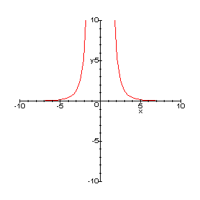 |
I have the students plot this
function, using convenient values (i.e. K = 10) to see how similar
the curve is to the photograph.
I remind students that the domain of a polynomial curve
like our original parabola is boundless, whereas actual radii are only
positive. The inverse function is respectfully undefined at r =
0.
|
Returning to the decision to use syrup, we brainstorm to
conclude that syrup 1) tastes better, 2) is easier to photograph, 3) is more
viscous than water and would provide a slower initial velocity. The smaller
v0 in
(4) and resulting smaller
K in (5) provides a more noticeable curve for given r0.
Syrup also reduces the effect of standing waves, clearly visible in the
photographs above. (I don't know what causes the standing waves – but I think
it's important for a teacher to leave some questions unanswered.)
I stress that inverse fourth model is still only a good
approximation. We have not accounted for the standing waves, air resistance,
measurement errors, and more. We can now deal with similar laminar flows in a
general way, and what we have may be suitable for most applications, but is
still flawed to some degree. As mathematicians, we should endeavor to evaluate
that error. (We have not done that in my high school class, but I emphasize the
need to do it someday.)
Finally, I ask the students to ponder the usefulness of our
discovery. I suggest possible engineering situations where it might be important
to predict surface area or volume.
The experiment I outlined here takes 40 minutes to pull off.
After witnessing some of the remarkable claims by college students regarding the
meaning of the "regression" technique, and the confusion within high school
classrooms as to its purpose, I think this is time well spent.